
Segmentation algorithms to detect compositionally homogeneous domains
This page is a companion for the paper on comparative testing of DNA segmentation algorithms using benchmark simulations, written by Eran Elhaik (me), Dan Graur and Kresimir Josic. The intention is that this page will host the implementation of the Jensen-Shannon divergence algorithm we describe in the article. For now, we present the file version that we wrote in Matlab, but our hope is to eventually host versions in a variety of languages. In general, we want to make the methods as accessible to the community as possible.
Convert DNA sequence to Xbp file
This bash script accepts a DNA sequence (no headline). It then count the GC nucleotides per a certain
window size (default is 32bp). The output file is in the format of Xbp and is the input file for the IsoPlotter algorithm. Usage
information is included in the file and can be viewed using any text editor.
CalculateGCWindow.n (Bash)
Example: Readme, Input, and Output
Algorithms
We tested seven segmentation algorithms from the literature. Below, we describe only the main ideas behind each algorithm. In most cases,
the details and the implementation are presented in the original papers. We could not obtain the original code for one of the programs, and
reconstructed the program to the best of our ability on the basis of its description. For many several algorithms, it is unclear which
parameters we were to use under which circumstances. In such cases, we used the default parameters recommended by the authors. Unless
obtained from the authors, algorithms were implemented in Matlab 7.5.
1. Partition sequence file (Xbp format) using the DJS algorithm
This function implements the Jensen-Shannon divergence algorithm (DJS) as
described in our paper. In this method, sequences are recursively partitioned by maximizing the difference in GC content between adjacent
subsequences, as measured by the Jensen-Shannon divergence statistic (DJS) (Lin 1991). The DJS statistic is calculated over all possible
partitioning points and the sequence is partitioned at the position of maximum DJS. The process of segmentation is terminated when the
maximal DJS value is smaller than a predetermined threshold of 5.8·10–5. Usage information is included in the file; type 'help
DJSSegmentation.m' at the Matlab prompt for more information.
DJSSegmentation.m (Matlab)
2. Partition sequence file (Xbp format) using the DJS BIC algorithm
DJS BIC. In this method (Li 2001a; Li et al. 2002) sequences are recursively partitioned by maximizing the difference in GC content between
adjacent subsequences measured by the Jensen-Shannon divergence statistic (DJS) (Lin 1991). The “segmentation strength” s is a predefined
measure of stringency for the segmentation that considers the sequence length and the maximum DJS value (for full description see
Supplementary Materials). The process of segmentation continues as long as s is larger than a predetermined threshold s0. We used s0 = 0.
DJSBICSegmentation.m (Matlab)
3. Partition sequence file (Xbp format) using the H&M algorithm
In Haiminen and Mannila’s (2007) method, the sequence is partitioned into
100 kb non-overlapping windows and their GC content is calculated. The algorithm divides the sequence into a predetermined number of
domains (k) so that the sum of squares of the Euclidean distance between the GC content of the segments and the sequence GC content is
minimized. A serious disadvantage of this algorithm is its quadratic computation time, which precluded the testing of its performance on
long sequences (= 100 kb). In addition, determining a realistic value for k, as far as real-life sequences are concerned, is not a
straightforward task; however, in our simulation sets, it was simply the number of predetermined domains. We used the segmentation code
provided by the authors at http://dx.doi.org/10.1016/j.gene.2007.01.028
4. Partition sequence file (Xbp format) using the Sarment algorithm
This package implements an algorithm that partitions the sequence into
k domains using maximal predictive partitioning (MPP) (Guיguen 2005). As in the previous case, the final number of domains (k) has to be
determined a priori. Again, in real-life situations, the value of k is unknown; however, in our simulation the value of k is known. We used
the segmentation code (version 4) provided by the authors at http://pbil.univ-lyon1.fr/software/sarment/ (file tar.gz).
5. Partition sequence file (Xbp format) using a sliding-window algorithm
We used the sliding-window algorithm as described by Costantini et
al. (2006). In this method, the sequence is partitioned into 100 kb non-overlapping windows. The GC variation within every window is
calculated by the GC content standard deviation. The windows are scanned for differences in the standard deviation between every two
adjacent windows. Adjacent windows with differences between their standard deviation below a given threshold of 1% were considered
concatenated domains (Costantini et al. 2006). We did not observe any cases that would justify using smaller thresholds.
CostantiniSegmentation.m (Matlab)
6. Partition sequence file (Xbp format) using the Compositional heterogeneity index
This method (Nekrutenko and Li 2000) uses a divide-
and-conquer approach (see, Cormen, Leiserson, and Rivest 1990). The sequence is partitioned to n windows of length l, and the CHI measure
is calculated for each window. Sequences are then recursively partitioned by maximizing the difference in GC content between adjacent
subsequences, measured by the CHI measure
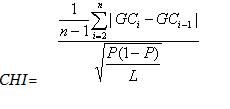
where the GC content of each nucleotide in the window is GCi and the mean GC content of the window is P. The process of segmentation is terminated when the maximized CHI is smaller than a given threshold. In order to estimate the halting threshold parameter, one hundred thousand random sequences, each 1 Mb long, were drawn from a uniform distribution. Each of these sequences was partitioned into two at a random point, and the CHI value for each segment was calculated. We followed the procedure of Cohen et al. (2005) and chose a CHI value corresponding to the upper 5% of the cumulative CHI distribution. We tested a wide range of window sizes (l = 2, 3, 4, 5, and 10). The algorithm appeared to perform best with window sizes of 2.
ChiSegmentation.m (Matlab)
7. Partition sequence file (Xbp format) using the IsoFinder algorithm
We unsuccessfully tried to obtain the code for this program (Oliver et al. 2004) from the corresponding author. As an alternative, we
reconstructed the IsoFinder algorithm to the best of our understanding of the description in Oliver et al. (2004). In this method, the
algorithm uses a sliding-pointer that moves from left to right of the sequence. At each point, the mean GC contents to the left and the
right of the pointer are compared using the t-statistic. At the maximum t-statistic point (tfilt), the algorithm compares the two
subsequences to the left and to the right of the point as follows: both subsequences are divided into windows of size l0 and their window
GC contents are compared using Student's t-test to obtain tfilt. The distribution of tfilt values [P(t = tfilt)] was obtained using Monte
Carlo simulations (Bernaola-Galvבn et al. 2001). The statistical significance P(t) of the possible partitioning point with tfilt = t is
defined as the probability of obtaining the value t or lower values within a random sequence. If the significance of P(t) exceeds a
selected threshold P0, the sequence is partitioned at this point into two subsequences and the procedure repeats recursively. We followed
Oliver et al. (2004) and used l0 = 3000 bp and P0 = 95%.
IsoFinderSegmentation.m (Matlab)
Download all files
To easily get the most updated versions of the files including sample input and output files, they are available as a
downloadable zip file here. Download all files